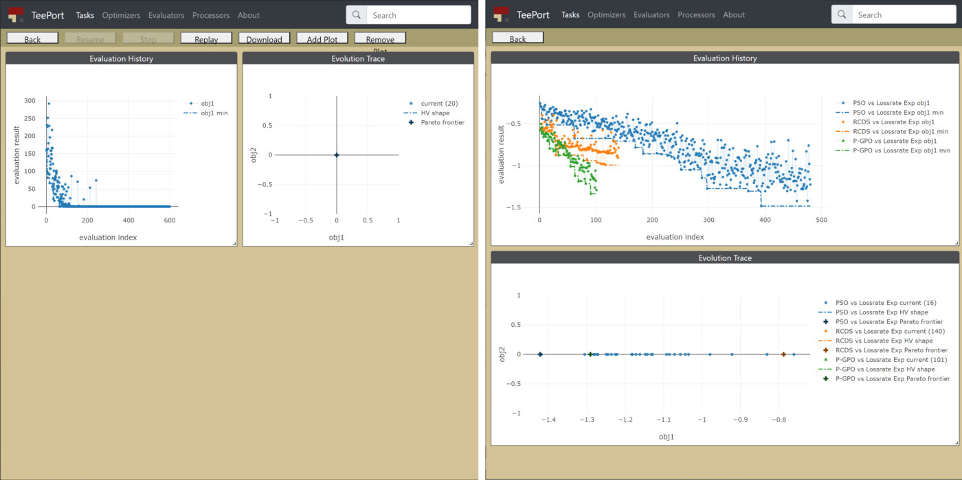
At an accelerator like SPEAR3 the optimization problem lives in the control room, usually as a Matlab script that sets some magnets and reads the beam back. The algorithms live on laptops, a lot of them in Python. Trying a new one meant cloning it onto a control-room computer and wiring it to the script by hand, and setting up its environment there often needed admin rights (the setup could also break the control system's own configuration). Then the next one, same thing again. I wanted to run the optimizer from where it already was and leave the script alone, so I came up with Teeport. I wrote the server, the dashboard, the plugins and most of the adapters at SLAC from 2019 to 2021, and Xiaobiao Huang, Minghao Song and I wrote it up in Frontiers in Big Data in 2021.
- 2 linesof your code to change, in the typical case, to put an algorithm or a problem on Teeport
- 6functions in the whole API
- 2labs where it was tested and deployed, SLAC and ANL
The wall
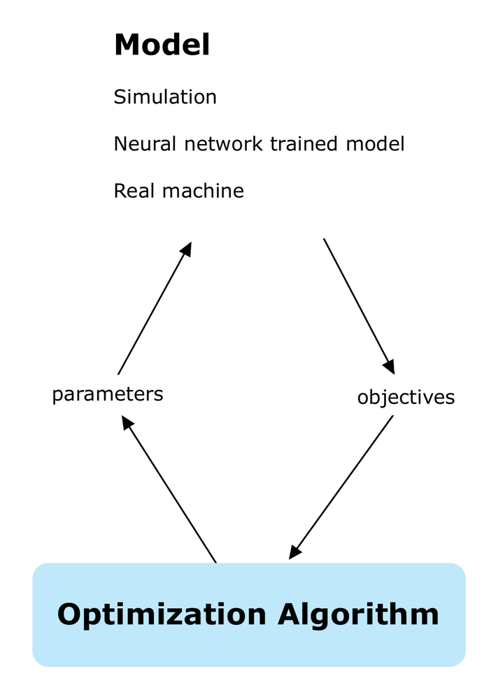
In my 2020 slides it was a brick wall with three words on it. Distance and language are the laptop and the Matlab from above, and confidentiality is about the script. An evaluation script can hold the token for the control system, or knobs you would rather nobody else saw, so it should stay where it is. Teeport leaves the code on both sides alone and only moves data through the wall, mostly X (the settings to try) one way and Y (what was measured) the other.
run_ and use_
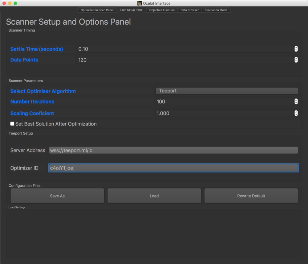
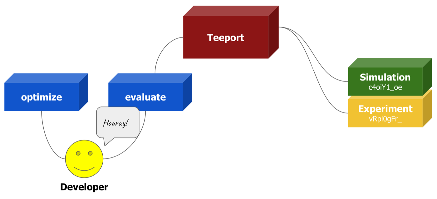
Take that Matlab script. To Teeport it is just a function, Y = evaluate(X). An algorithm is a function that takes one of those, optimize(evaluate). In the control room, teeport.runEvaluator publishes the script and gives you an id. On a laptop, use_evaluator takes that id and hands back an ordinary local function:
from teeport import Teeport
teeport = Teeport('ws://localhost:8080/')
evaluate = teeport.use_evaluator('c4oiY1_oe')
Your optimizer calls it like any other function. It looks local. The measurement still happens in the control room, and whoever published the script decides when it runs, so your optimizer cannot reach the machine except through it. Optimizers get the same pair of calls, so someone with a problem can borrow an algorithm by id.
The hidden optimizer
use_evaluator took the most work (it lives in the Python client). On the server every run is a task, and a task needs an optimizer client, a function that keeps running and produces X. Here there is no such function, just your loop calling evaluate(X) whenever it likes. So your first call quietly starts a private optimizer inside the client and creates the task. Its loop never ends. It waits on a future for the next X, sends it out, and puts the Y that comes back into a second future, the one your evaluate(X) is waiting on. To you it is a blocking function, so an existing algorithm can work on a remote problem unchanged.
The pending queue
The server is a small Node.js WebSocket service, and it does as little as it can. Before SLAC I had written the same kind of server at Visual3D, the one every headset and workstation in a mixed-reality navigation system talked through. Teeport's server passes X to the evaluator and Y back to the optimizer, and anyone watching gets a copy of Y. It also keeps the history. Every X lands in a pending queue first and goes on only if the task is running. That one check is all there is to pause and resume. Pause, and the batch waits. Resume, and the server replays the queue to the evaluator. Neither the algorithm nor the problem finds out, and neither side had to add a line of code for it.
All of it lives in memory. A run survives a server restart only if somebody exported it to JSON first. I drew an archive database behind the server and a rollback to an earlier point in a run, and neither got built.
The dashboard
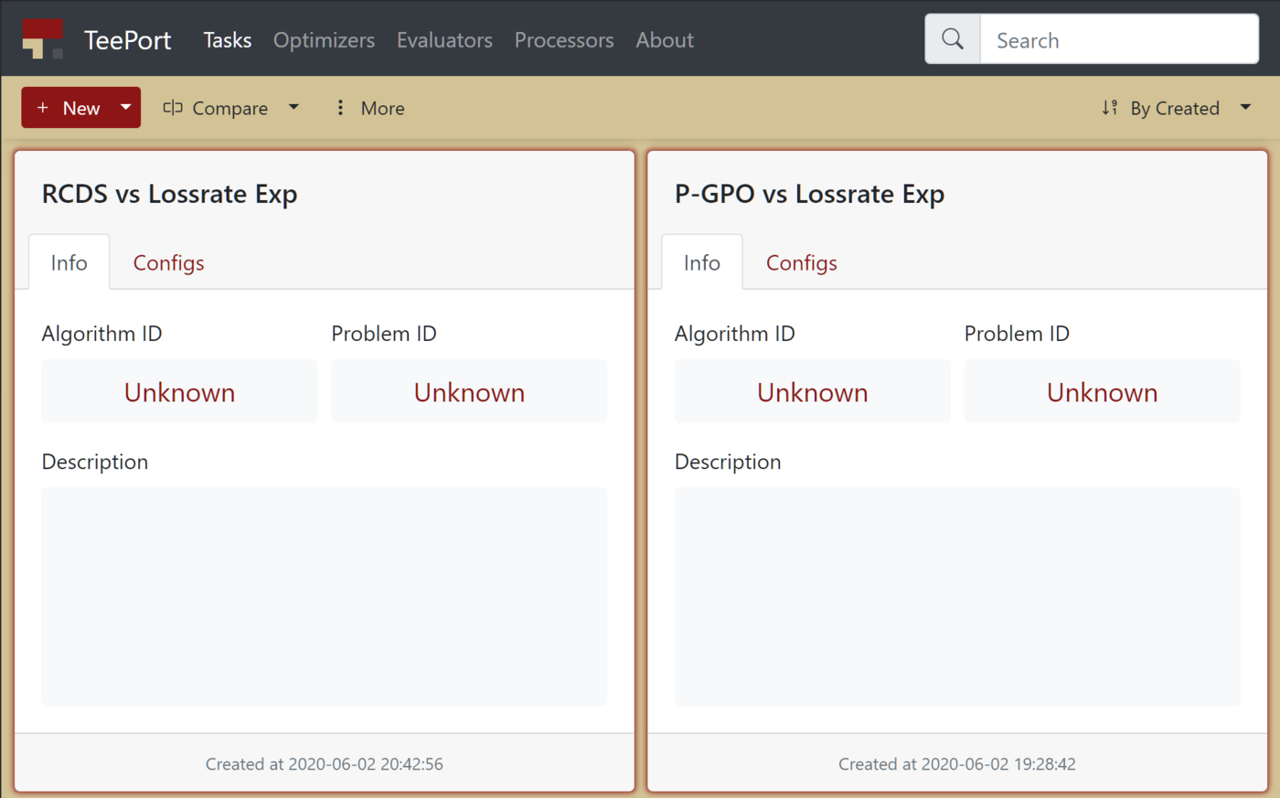
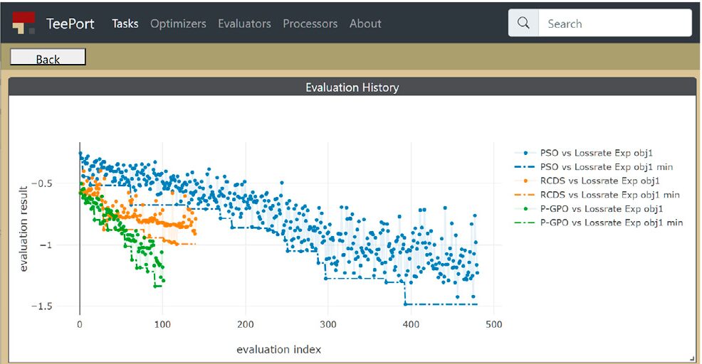
The dashboard (React and Plotly) is one more client. A task page subscribes as a monitor that asks for Y only, so the server blanks X in every generation before sending, and X comes down when you download the run. That was for big problems. NSGA-II on a 500-dimensional problem piles up about a gigabyte of history by the time it converges, and a browser tab will not hold that. You pick runs in the task list and press Compare to overlay them, even while some are still going, or benchmark an optimizer over repeated runs.
On SPEAR3
The three of us used it on storage-ring optimizations at SPEAR3, and Minghao, our first user, had tested the prototype and written part of the Matlab adapter. In our January 2021 report to SSRL we wrote that most of the online optimizations in it, simulated and on the ring, ran through Teeport, the loss-rate runs above among them. We published it from a Matlab session in the control room and optimized it from a laptop. A run could go against the simulated ring first and then the machine, by changing one id.
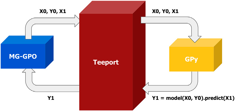
The wall turned up inside one algorithm as well. MG-GPO is Xiaobiao's algorithm (Minghao and I developed it with him), and it is written in Matlab. We could not find a good Gaussian-process package for Matlab, and Python had GPy. So GPy ran as a Teeport processor (a stateless helper either side can call), teeport.useProcessor gave the Matlab code a predict function, and everything else stayed in Matlab. How the tuning went is on the MG-GPO page.
After Teeport
Teeport was good at remote runs and at benchmarking algorithms. Hands-on tuning in the control room needed something else, and in 2021 I started Badger for that. The public instance at teeport.info still loads. Its task list is empty, since everything lived in memory.
Sources are the paper (Zhang, Huang and Song, Frontiers in Big Data, 2021), our report to SSRL (Huang, Song and Zhang, January 2021), my 2020 slides and the public SPEAR3-ML repositories.