Tuning jobs in the control room used to be scripts. Somebody glued an algorithm to one problem, wrote the progress plots yet again (dull code, but you do need to watch the run), and once it was going there was no clean way to pause it. The next job got a new script. I started Badger at SLAC in 2021 so all of that would be one program. You pick a machine and some knobs, say what to watch, choose an algorithm and press Run. I led it through 2025 and wrote the IPAC'22 paper about it with colleagues at DESY and BNL.
- 7+facilities that adopted it, in the US and Europe
- 15 minfor ESRF's lifetime tuning with TuRBO in Badger, about a seventh of what their run-by-hand scan script took
- 20 to 30 minfor the SLAC team to halve the injector emittance in both planes at LCLS and LCLS-II
Environments and routines
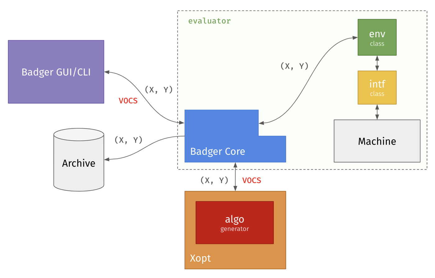
Take LCLS. The environment I wrote for it in 2021 has tens of magnets you can move and readings like the FEL pulse energy and the beam size. That's the machine, described once. A routine picks a few knobs and a reading or two from it, sets the ranges, adds an algorithm, and gets saved, so next time it's one button. Under the environment sits an interface, the only code that talks to the control system (EPICS, DOOCS or Tango, and a toy problem can skip it). Why split it like this? Operators change a routine a little all the time, and nobody should have to open the environment's code for that.
At first Badger had its own algorithm plugins and reached Xopt through an extension. For 1.0, in December 2023, I rebuilt the core so Xopt drives every run. Xopt is a SLAC library other people lead, and it owns the algorithms (TuRBO among them) and proposes each next point. Badger takes the point to the machine and brings the reading back, and it keeps every step on screen and on disk.
The window
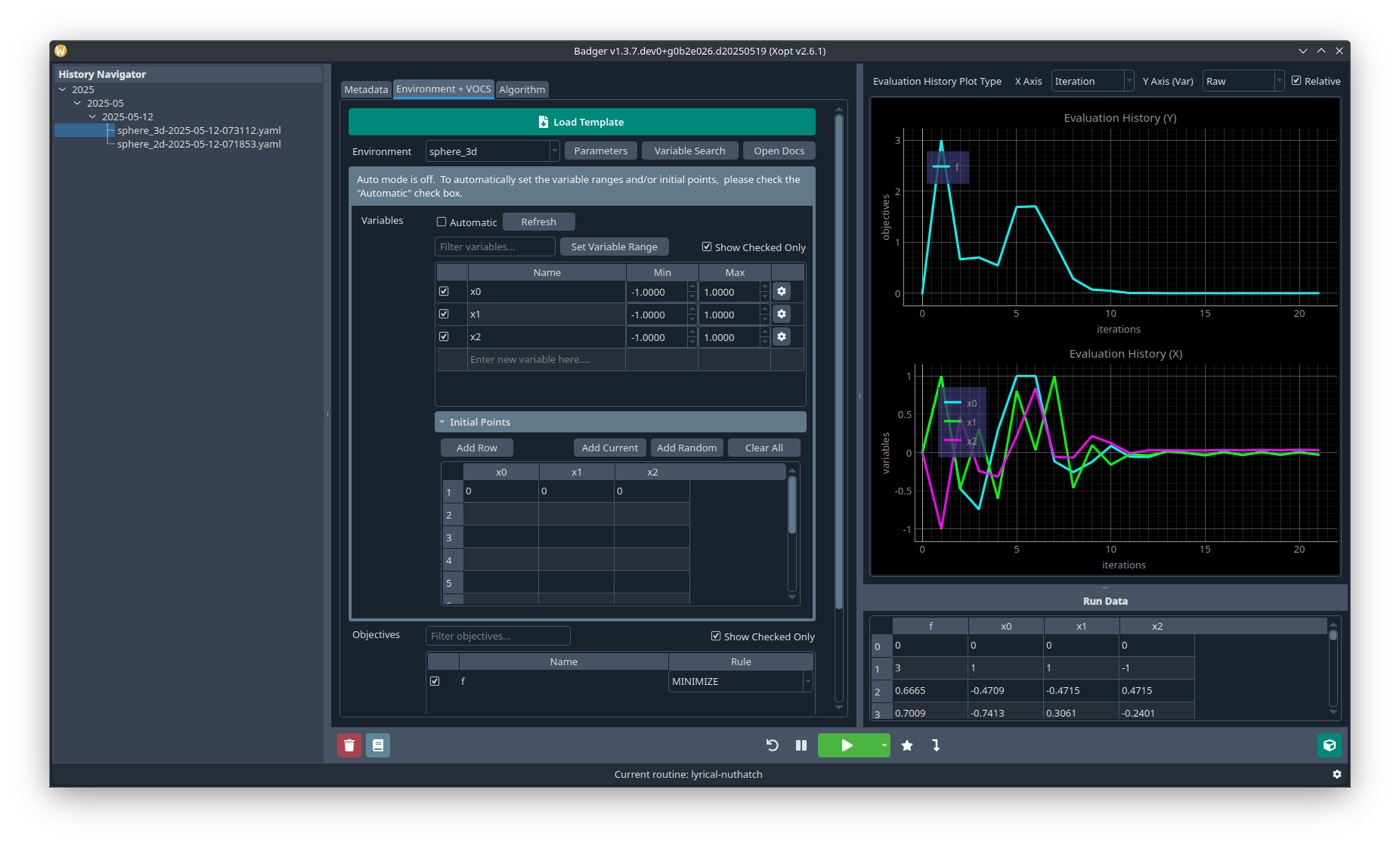
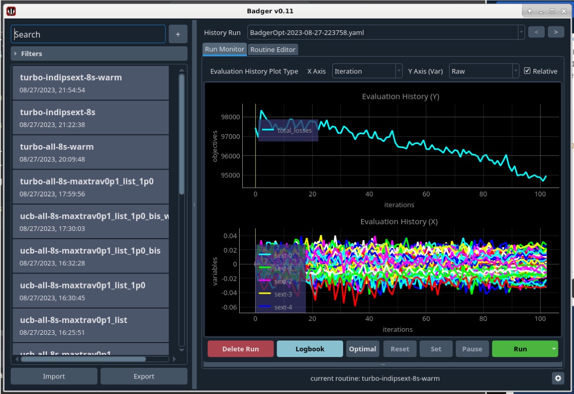
Most people meet Badger as the window below. A few pieces of it I added along the way. Since 2023 a run in progress is written to disk every second, so a crash doesn't take it along. In early 2025 I rewrote the GUI for 1.3.0 and dropped the database. Each run is now a YAML file in a folder for its day, and you can read it in any editor. You can also add an objective or a constraint while a run is going.
It only officially runs on Linux. From 1.3.0 on, the command line only partly works. Every facility still writes its own environment. Besides SLAC, ESRF and DESY, it has been used at BNL, Argonne, Fermilab and KIT, and KIT forked Badger into their own GitLab and runs it from containers. At LCLS one photon beamline team wanted plots built for their problem and went straight to Xopt.
Lifetime at ESRF
Some of the most useful runs happened in a control room that wasn't ours. ESRF and DESY had first tried extremum seeking on their storage rings and found it hard to tune. Then they switched to Badger. ESRF's Tango interface was, in their words, "mostly a copy of the existing Badger examples". Changing two lines moved it between the ring and their simulator. They spent no machine time debugging. ESRF's team ran all of it. I wrote the Badger section of their paper.
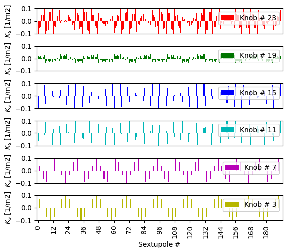
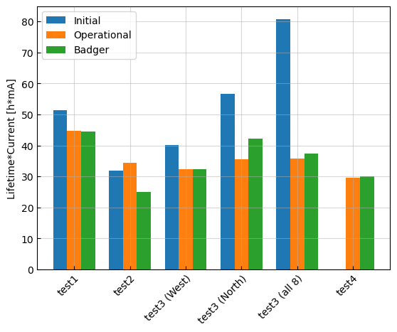
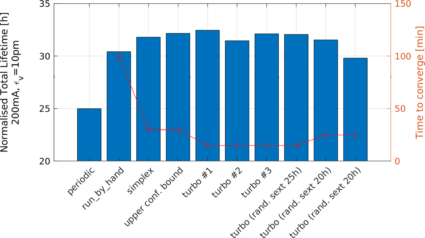
The job was the ring's lifetime. A knob there moves all the sextupoles at once in one pattern (all the focusing ones following a cosine around the ring, for example). They kept 24 sextupole knobs and 4 octupole knobs, and the objective was the total loss over the ring's loss detectors. Their usual tool was a script that scans one knob, fits a parabola, keeps the best amplitude and moves to the next. Through Badger, simplex and UCB converged in about half an hour, and Xopt's TuRBO faster still, with the smallest loss swings along the way. The best setting gave a record Touschek lifetime of 41 ± 11 hours. When random sextupoles knocked the lifetime down to 20 hours, TuRBO brought it back near the operational best. In 2023 ESRF made Badger with TuRBO available to operators during user service.
Injection at ESRF, coupling at PETRA III
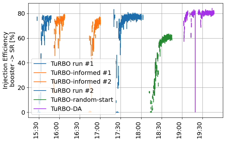
Injection efficiency was a separate campaign. The first runs moved the transfer-line quads, septa, kicker and timing, and a later one moved 17 knobs for dynamic aperture. Each point was the average of ten injection shots, to spare the hardware and keep the stored current under its limit. Against the old user-mode settings, efficiency went from 65 to 75 percent. Not every run worked. One started from random quad settings and stalled near 60 percent, and warm-starting TuRBO from an earlier run's data showed no clear gain.
PETRA III was a draw. It got one machine-study shift in March 2022, minimizing coupling. Badger's runs came out about level with the operational settings, and starting from those settings it found nothing better. DESY kept it for machine studies and for their PETRA IV upgrade work.
LCLS
At SLAC I ran all of Badger's beamline testing at LCLS until the summer of 2025. LCLS-II commissioning used it too. What the SLAC team had by then is in our ICALEPCS'25 paper. The team tuned injector emittance with it on a handful of injector knobs. FEL tuning moves some or all of the matching quads (up to about twenty) with beam loss capped. That way the team routinely brought pulse intensity up from a cold start. After the 2025 summer downtime both LCLS and LCLS-II restarted with Badger tuning in the procedure, and the routines were saved as templates for the next restart.
The cli-run branch
Since late 2025 I've kept adding one thing, a way for another program to drive the Badger window. Otter needed it. It lives on the public cli-run branch, and it hasn't been merged. You can launch the window with a routine and have it start on its own. Drop a new routine file at a watched path and the window stops, reloads and runs again in place, and each evaluation also goes out as one JSON line to a log. A stop file stops the run the same way the Stop button does, and the window stays open. Before, the only way to stop it from outside was to kill the process, window and all, so every round of a campaign paid for a fresh start of the GUI. The branch also makes headless command-line runs work again, with pause and resume.
Everything goes through files, so there's no port to open and nothing to log in to, and it works the same over ssh. One Qt detail needed a second pass. The file watcher quietly forgets a file when an editor saves it by writing a temporary file and renaming it, so the window watches the folder too and adds the file back after every change. All of it is opt-in. Without the flags Badger behaves as it always did.
Sources are our IPAC'22 paper (Zhang et al., 2022), ESRF and DESY's ICALEPCS'23 paper (Liuzzo et al., open access under CC BY 4.0, where the architecture and ESRF figures come from), our ICALEPCS'25 paper on Xopt and Badger (Roussel et al.), and the xopt-org/Badger repository with its docs and cli-run branch.