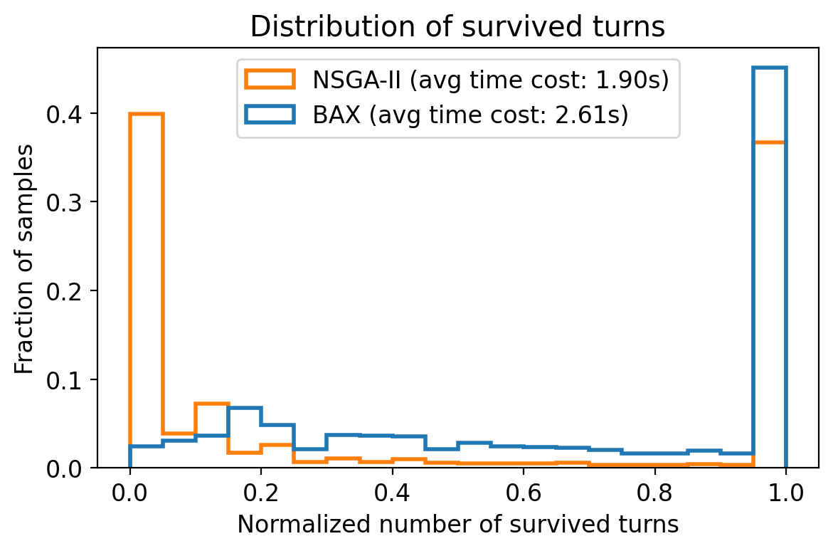
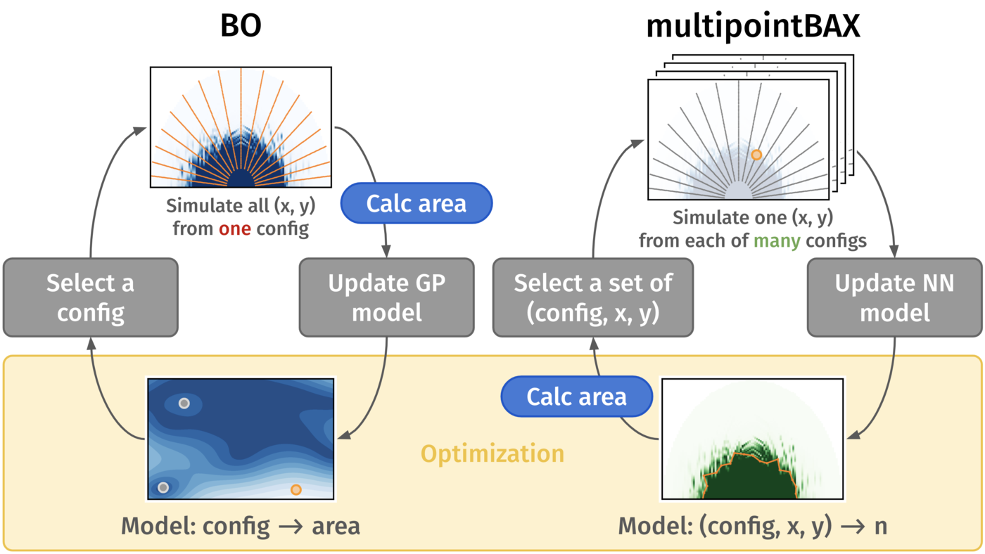
To see how big a storage ring's dynamic aperture is, even in simulation, you launch a couple of thousand particles, track each for thousands of turns and count the survivors. That's one sextupole setting. A genetic algorithm wants this for every candidate, so a design study typically stops at around a thousand designs. Multipoint BAX tracks one particle per simulation instead. It picks the particle near the predicted edge of stability, in a setting the model predicts is near the best, and a neural network learns the whole map from those. I first-authored the paper (seven of us, from SLAC, DESY, LBNL, USC and Jefferson Lab), and it came out in Physical Review Accelerators and Beams in September 2026.
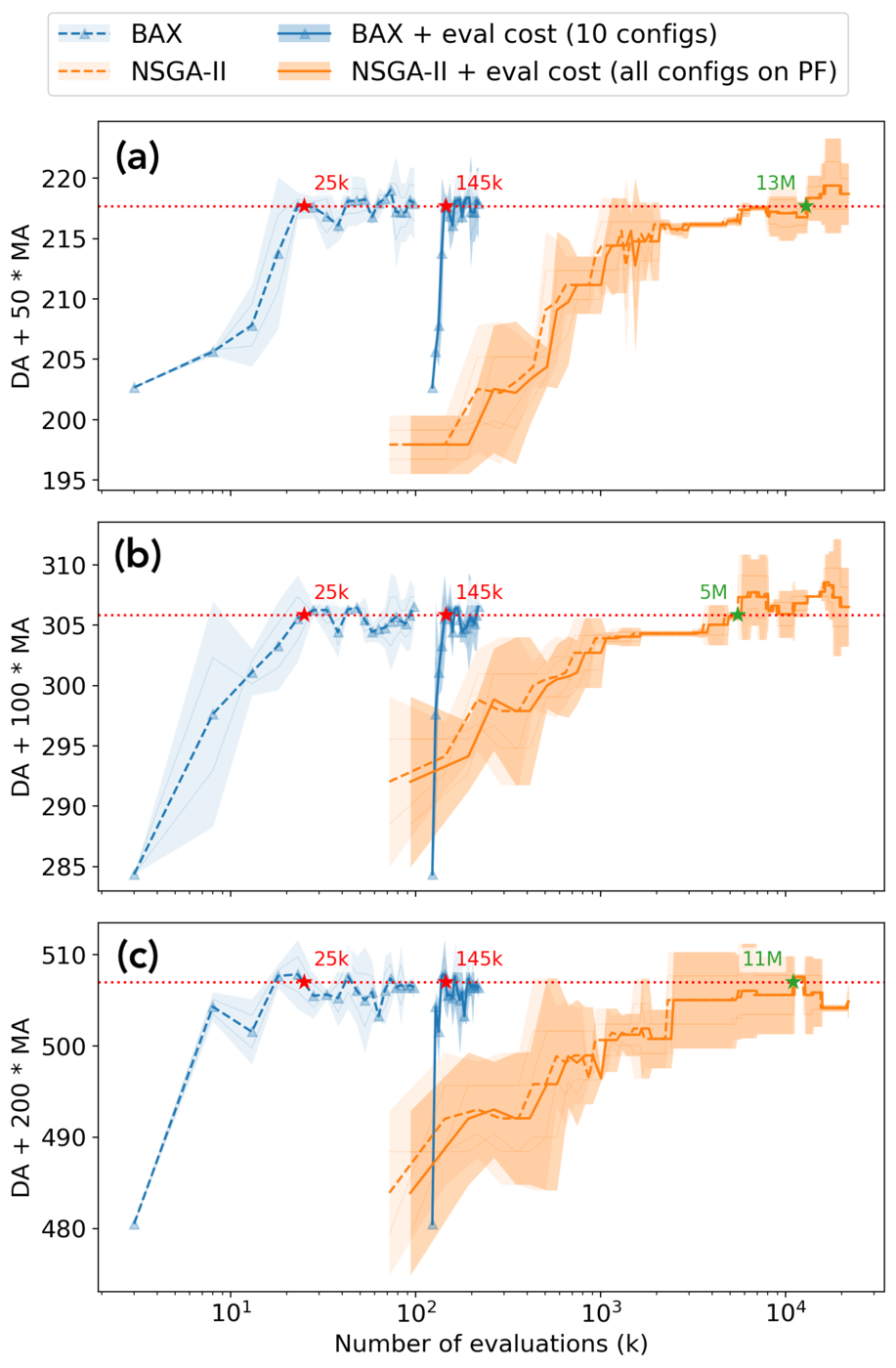
- 40×fewer tracking simulations than NSGA-II for the same hypervolume, final check included
- >400×fewer simulation calls inside the optimization loop alone
Two areas per setting
Dynamic aperture (DA) is how far off the orbit a particle can start and still stay in the ring, which decides how much injected beam gets caught. Momentum aperture (MA) is how big an energy error it survives, and that sets the lifetime. Sextupoles shape both. Pushing one usually costs the other. So you're after a Pareto front, and each point on it is two maps of tracked particles boiled down to two areas.
Bayesian optimization tries fewer settings (the paper counts MG-GPO, Xiaobiao Huang's method that I helped develop, among the earlier attempts), but it still pays a full map for each one. Multipoint BAX models one level down, from setting and starting point to turns survived, and runs the design algorithm on that model. The method isn't mine. BAX is Neiswanger, Wang and Ermon's, multipoint BAX is Miskovich and others' (Neiswanger and Ratner, two of my co-authors, are on it), and our paper applies it to DA and MA.
The loop
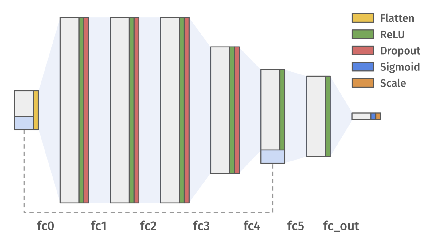
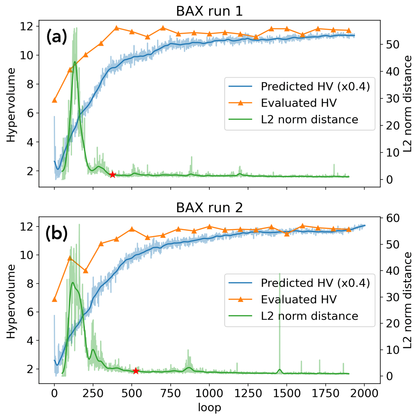
A full 2,000-loop run piles up more than 100,000 tracked particles, far too many for a Gaussian process. So the model is a neural network that takes four knob values and a starting position and returns the fraction of turns survived (one network for DA, one for MA). We pretrain both on 3,000 random single-particle runs. Every loop then runs NSGA-II on the networks to predict the front, which is cheap because nothing gets tracked. Two conditions then fix the pool we may track from. The setting has to be one we kept near that predicted front, and the starting point has to be one the network puts in a band around the edge of stability.
The MA network gets the same treatment, with a band of its own. That leaves roughly 2,500 candidates. Fifty of them, drawn at random, go to pyAT, and the networks get finetuned on the results.
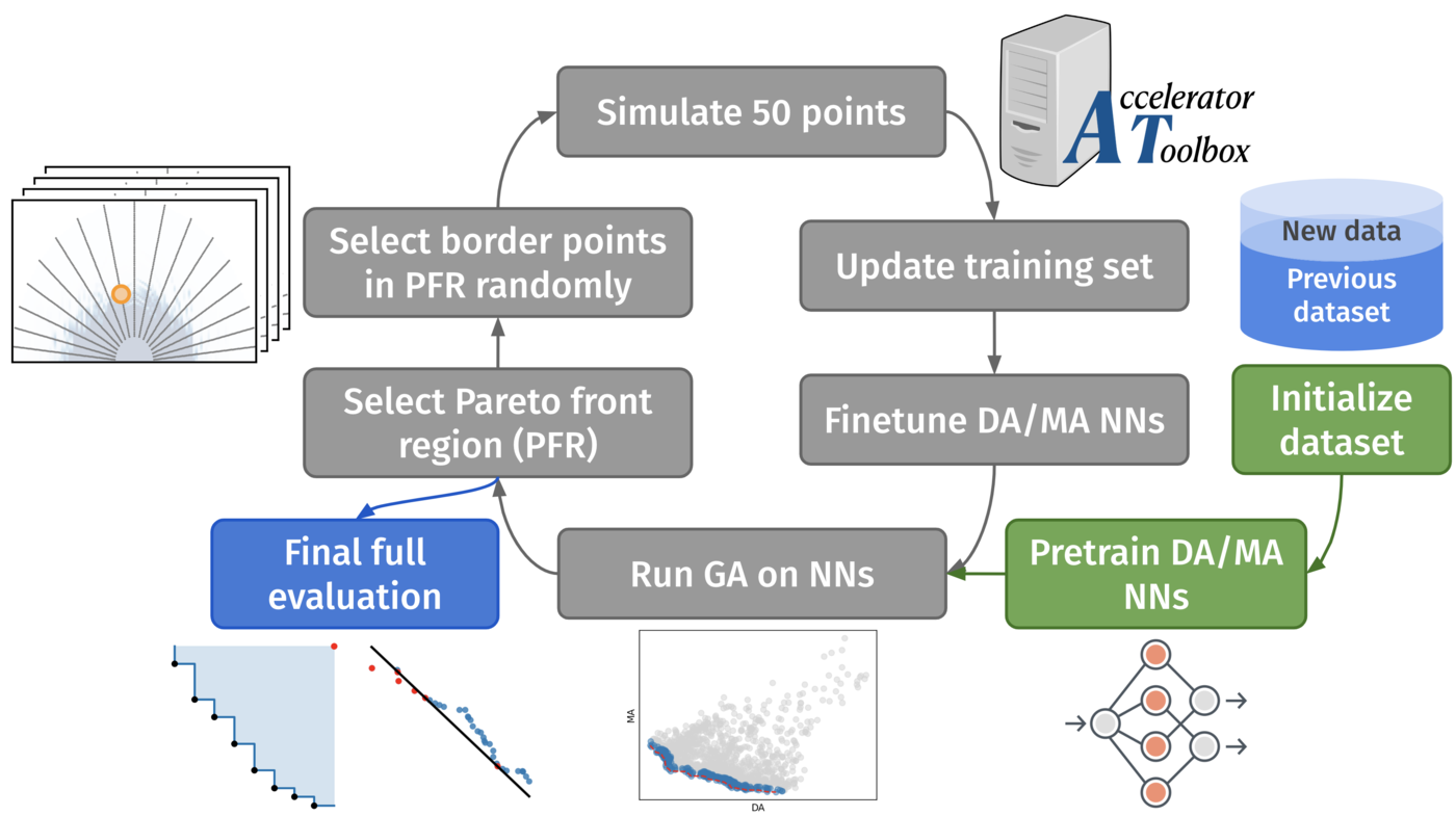
It's cruder than the name suggests. With one deterministic network and the greedy MeanBAX rule (Chitturi and others), nothing carries an uncertainty. The batch is a random draw where joint mutual information would be smarter. We hardly tuned the hyperparameters either.
SSRL-X
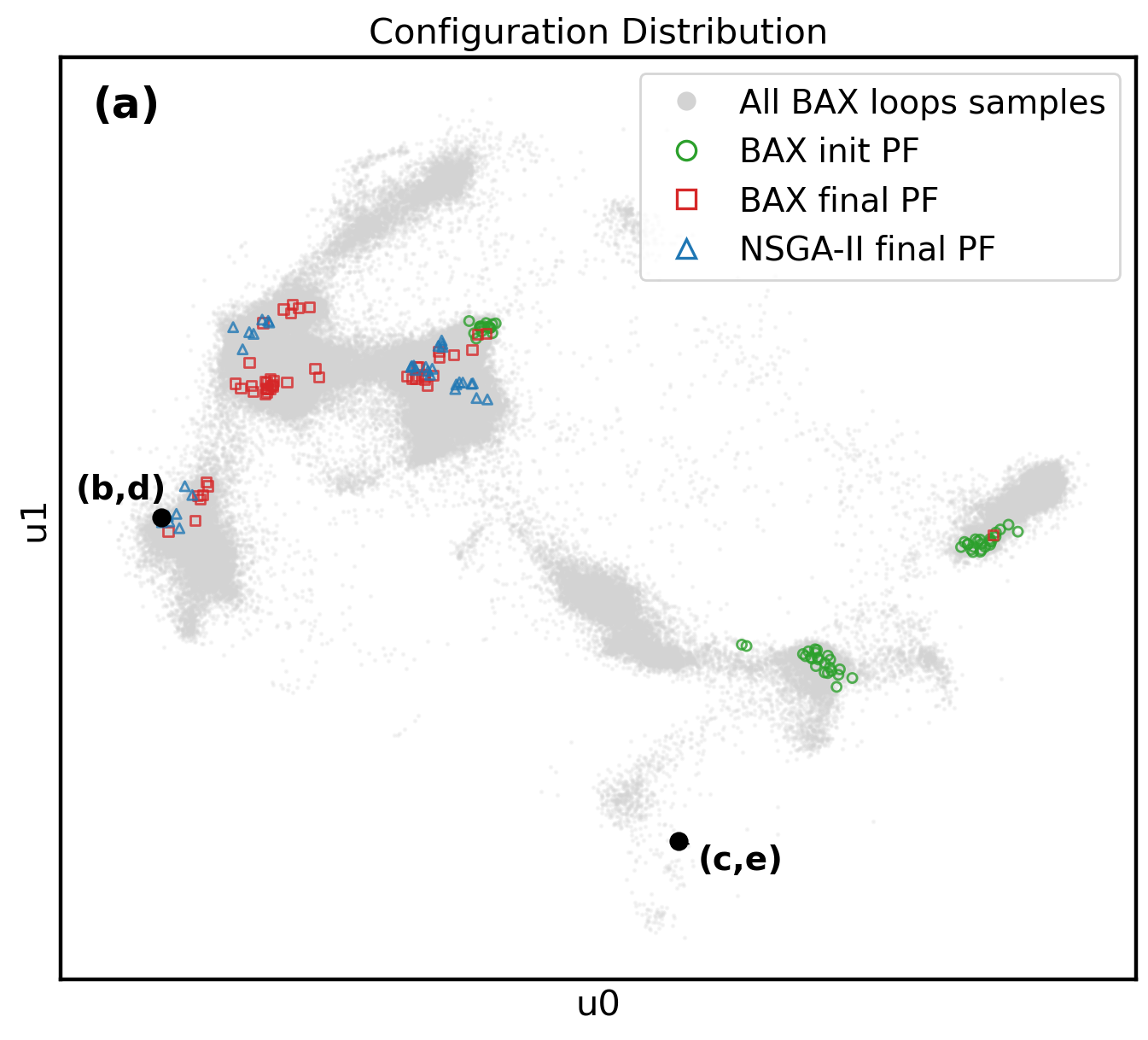
The test case is SSRL-X, a low-emittance lattice that's one option for a future SSRL upgrade (Raimondi and others designed it). Following Huang and Safranek, its six sextupole families become four knobs that leave the chromaticity alone. Every simulator call drew one of ten error seeds at random. The final check used fresh ones.
Against NSGA-II
The baseline was NSGA-II, the same optimizer BAX runs on its networks, and we ran each method twice. You can't see the true hypervolume mid-run, so BAX's stopping rule watches the networks instead, and fires once their predicted front stops drifting from where it was 50 loops back. For BAX that came at about 25,000 simulations. We kept going past it anyway, and the stop lined up with where the true hypervolume had leveled off. NSGA-II reached the same hypervolume at around 11 million.
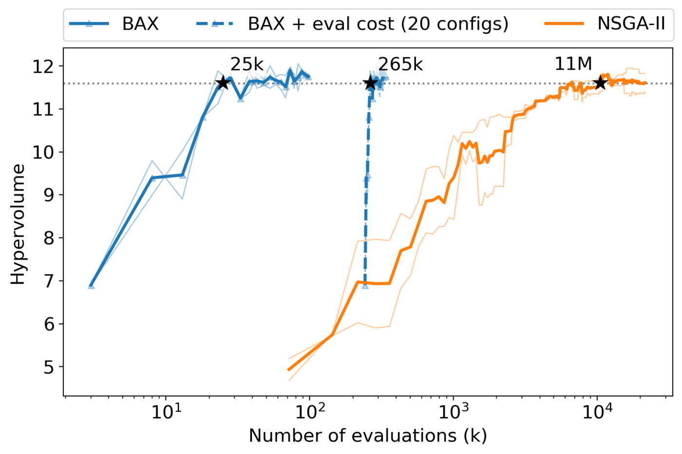
The gap between the two ratios up top is the final check. Only a tenth of BAX's simulations happened inside the loop. Tracking full maps of the chosen settings took the rest (partly because a four-knob search is easy), and on a harder problem that share would shrink.
What the network learned
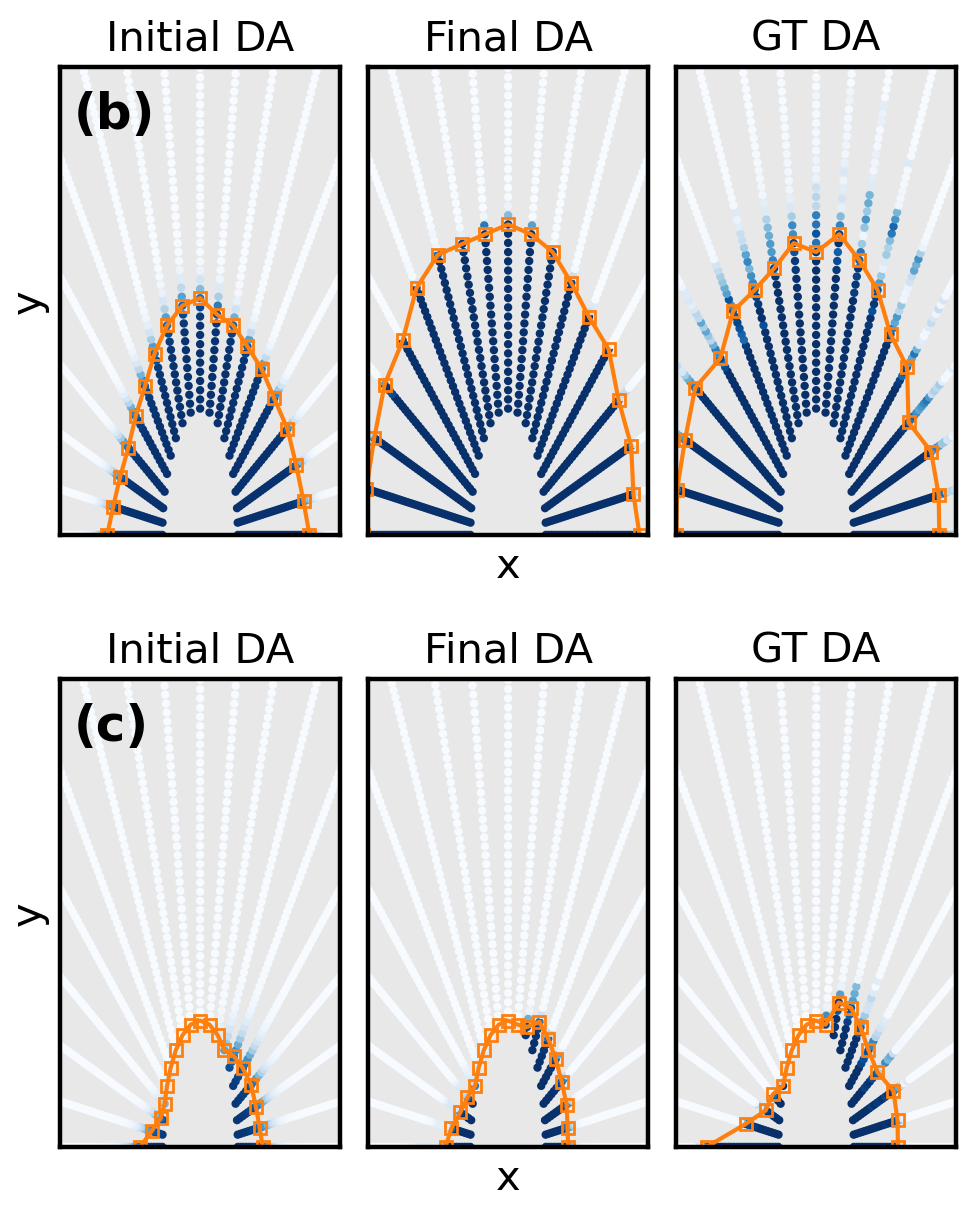
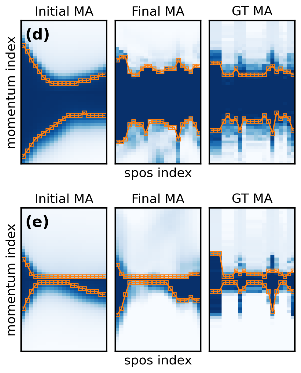
For a setting on the front, the network's first boundary was far too small, and by the end it had the right shape. For a poor setting it hardly moved, since BAX stops sampling a region once the model writes it off. And you get to keep the network. It draws the DA and MA maps for any sextupole setting, so you can turn the knobs by hand and watch the aperture move.
mpBAX
I later packaged this kind of loop as mpBAX. A whole experiment lives in one config, a dict or a YAML file, with an oracle and a model per objective. It checkpoints every loop, so a run can resume or roll back. The core needs only NumPy and PyYAML.
Agents on the loop
In 2026 we let LLM agents work on the optimizer itself, using LBNL's framework (autoresearch-commissioning, built by T. Hellert, one of the paper's co-authors). Our group was its first outside user. An agent proposes one change to the training script, and a separate reviewer agent reads the diff. The change then runs on a fixed tracking budget and gets merged only if the true hypervolume, tracked on a held-out error seed, goes up. We ran hundreds of experiments that way.
The cleanest test was a stricter benchmark. A search the agents can't touch picks which settings get scored. The surrogate ships crippled to a single linear layer that scores about zero. A validated three-layer MLP gets back to 10.80.
In the first pilot, the very first experiment spotted the underfit and rebuilt a three-layer MLP, landing on that number exactly. Nothing in the next 39 beat it. The second pilot passed it on its seventh experiment, reaching 11.40. The step that did it was a coarse-to-fine mask, wide while the surrogate is still noisy and tighter later.
These hypervolumes come from a separate benchmark with a smaller budget and its own scoring, so they don't compare with the paper's plot. The strict version has had only two pilot runs.
Published in Physical Review Accelerators and Beams (2026), doi:10.1103/4t6l-7jmg; preprint arXiv:2511.17850. Numbers and figures are from the paper and its supplemental material. The autoresearch numbers are from our internal campaign review.